Functional RCR Calculator
Input Data
Select Data Type:
Format: One data point per line: List the independent (x) values followed by the dependent (y) value, separated by white space. (In the case of multiple x values per data point, download and use the source code directly).
Weights, if unequal, should be included on the same line, separated by white space.
Alternatively, (symmetric, y) error bars may be entered instead of weights. These will be converted to weights using weight = 1/error2. However, if the scatter of the data is too large to be accounted for by the error bars alone, extrinsic scatter dominates and "Equal Weights" should be selected instead (§8.2.1, Maples et al. 2018).
Plot Data
Plot the data here, and zoom in (using the Box Zoom or Wheel Zoom tool) to the uncontaminated part of the distribution. Using the lower six buttons, you can change the basis of the data (in either or both x and y) such that the RMS scatter of average-weight data is approximately constant across the independent variable's domain, to be more compatible with RCR.
Model Data
Model y(x):
Here, select a function to model y(x), log y(x) or 10 y, depending on your chosen basis for y(x) in the above section. Depending on the chosen function, either x or log x will be displayed from the inputted data, depending on which model function is selected.
Next, in the box to the right, enter your guess for the model function parameters a0 , a1 , a2 , etc, one per line. For example, in the linear model case, a0 corresponds to the y-intercept, and a1 to the slope.
For large datasets and/or for non-listed custom functions,
it is recommended to just download the C++ source code (documentation included) here.
Suggested form of initial guess for x:
x = Σiwixi / Σiwi
Input Initial Guess for x:
Input Initial Guess for Model Function Parameters:
Model Bayesian Prior Distributions of Model Function Parameters (Optional):
Format: One model parameter per line. For each line, list the lower bound for the parameter (or an "x" if there is none), followed by the upper bound (or an "x" if there is none), followed by the mean and the standard deviation of the Gaussian (or two "x"s in their place if the prior is flat), all seperated by white space.
In total, each line will have four elements (either numbers or "x"s if no prior provided) seperated by white space. For example, a prior with lower bound of 0, no upper bound, and a Gaussian with μ = 1, σ = 2 would have a line of "0 x 1 2".
For custom priors, use the source code (with documentation included).
Input Priors:
Select Rejection Method
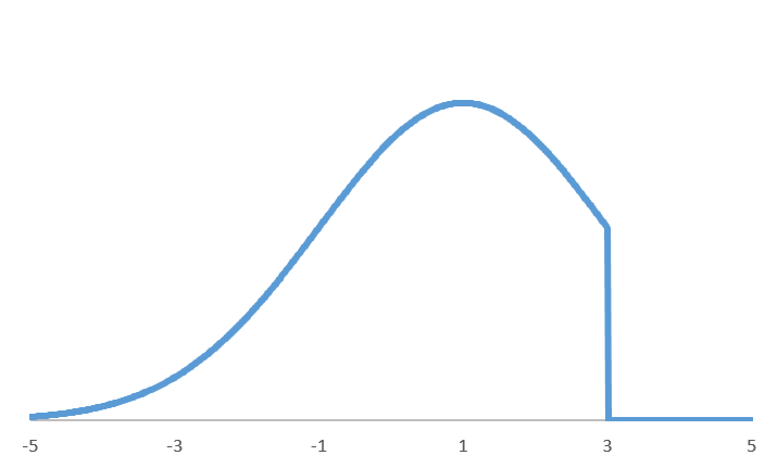
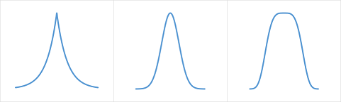
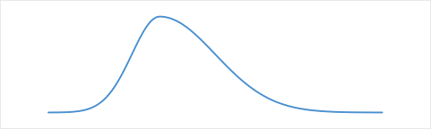
Select Uncontaminated Distribution about y(x):
Select Contaminant Type:
Selected Uncontaminated Distribution about y(x):
Selected Rejection Method:
μ: Median (§2.1; Maples et al. 2018)
σ : Broken-line technique (§2.2, §2.3)
Rejection proportional to σ both below and above μ (§3.1, §3.3.2)
μ : Half-sample mode (§2.1; Maples et al. 2018)
σ- , σ+ : 68.3%-Value technique (§2.2, §2.3)
Rejection proportional to min{σ- , σ+} both below and above μ (§3.2, §3.3.2)
μ: Half-sample mode (§2.1; Maples et al. 2018)
σ- , σ+ : Broken-line technique (§2.2, §2.3)
Rejection proportional to min{σ- , σ+} both below and above μ (§3.2, §3.3.2)
μ: Half-sample mode (§2.1; Maples et al. 2018)
σ- , σ+ : Broken-line technique (§2.2, §2.3)
Rejection proportional to σ- below μ and σ+ above μ (§3.3.1)
Fundamentally, RCR assumes that the uncontaminated distribution is Gaussian, or near Gaussian. In particular, our All High or All Low
and In Between
contaminant type options are especially sensitive to this assumption, and should not be used if this assumption is not met.
Note: Rejection method is iterative, preceded by iterative bulk rejection (§5), and proceeded by both (1) iterative "median + 68.3%-value technique" rejection, and (2) iterative "mean + standard deviation " rejection (§4).
Output
Note: results are in the chosen linear basis.
| Final model parameters and x: |
Selected points (x, y, and w if weighted): |
|---|---|