We have been developing three new, interrelated, statistical techniques. The first, Robust Chauvenet Outlier Rejection, or RCR, is advanced, but easy to use, outlier rejection. RCR has been published, with a full codebase and web interface completed.

The second, Trotter-Reichart-Konz Regression, or TRK, is a suite for worst-case Bayesian Regression in 2D. TRK was originally published as a Ph.D. thesis, and its codebase has been revamped in the form of an undergraduate thesis. We are preparing papers for journal submission and a web interface for it now, and the codebase is essentially completed.

The third, Parameter-Space Regression, or PSR, is an offshoot of both the aforementioned techniques, which we will be pursuing in the future; click here to learn more.

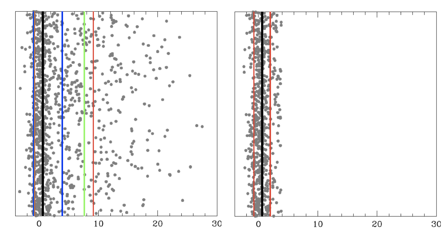
Left: data distribution heavily saturated with one-sided outliers/contaminants, with true value in black. Right: remaining uncontaminated distribution after single-value RCR outlier removal.

RCR is advanced, but easy to use, outlier rejection.

The simplest form of outlier rejection is sigma clipping, where measurements that are more than a specified number of standard deviations from the mean are rejected from the sample. This number of standard deviations should not be chosen arbitrarily, but is a function of your sample’s size. A simple prescription for this was introduced by William Chauvenet in 1863. Sigma clipping plus this prescription, applied iteratively, is what we call traditional Chauvenet rejection.

However, both sigma clipping and traditional Chauvenet rejection make use of non-robust quantities: the mean and the standard deviation are both sensitive to the very outliers that they are being used to reject. This limits such techniques to samples with small contaminants or small contamination fractions.

Robust Chauvenet Rejection (RCR) instead first makes use of robust replacements for the mean, such as the median and the half-sample mode, and similar robust replacements that we have developed for the standard deviation.

RCR has been carefully calibrated, and extensively simulated (see Maples et al. 2018). It can be applied to samples with both large contaminants and large contaminant fractions (sometimes in excess of 90% contaminated).

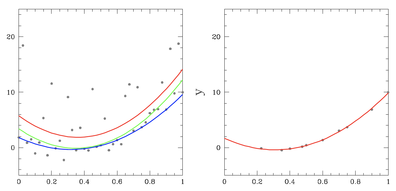
Left: Data distribution about true quadratic model (black), heavily saturated with one-sided outliers/contaminants. Right: remaining distribution after functional RCR outlier removal.

We have boiled it down to two simple user choices:

1. Are your uncontaminated measurements distributed symmetrically, like a Gaussian (or mildy peaked or flat-topped), mildly asymmetrically, or neither?

2. Are the contaminants to your measurements high and low in equal proportions, all high or all low, or something in between?

RCR can be applied to weighted data, to functional data (e.g., x vs. y), and we have incorporated bulk rejection to decrease computation times with large samples.

Try our online calculators (single value and functional), or download the source code and documentationhere or on our Github repo here. The source code is equipped with the maximum degree of customizability for using RCR, most notably with the functional form/model-fitting portion of the algorithm. In addition to the features offered by the online calculator, the full functional RCR source code also includes support for:

1. Running RCR on any custom model function with any number of independent ("x") variables and model function parameters;

2. Custom prior distribution functions for any or all of the model function parameters;

3. Support for model functions with custom "pivot point" variables that control correlation between model parameters, e.g. x0 for the linear model y(x)=b+m(x-x0);

and more.

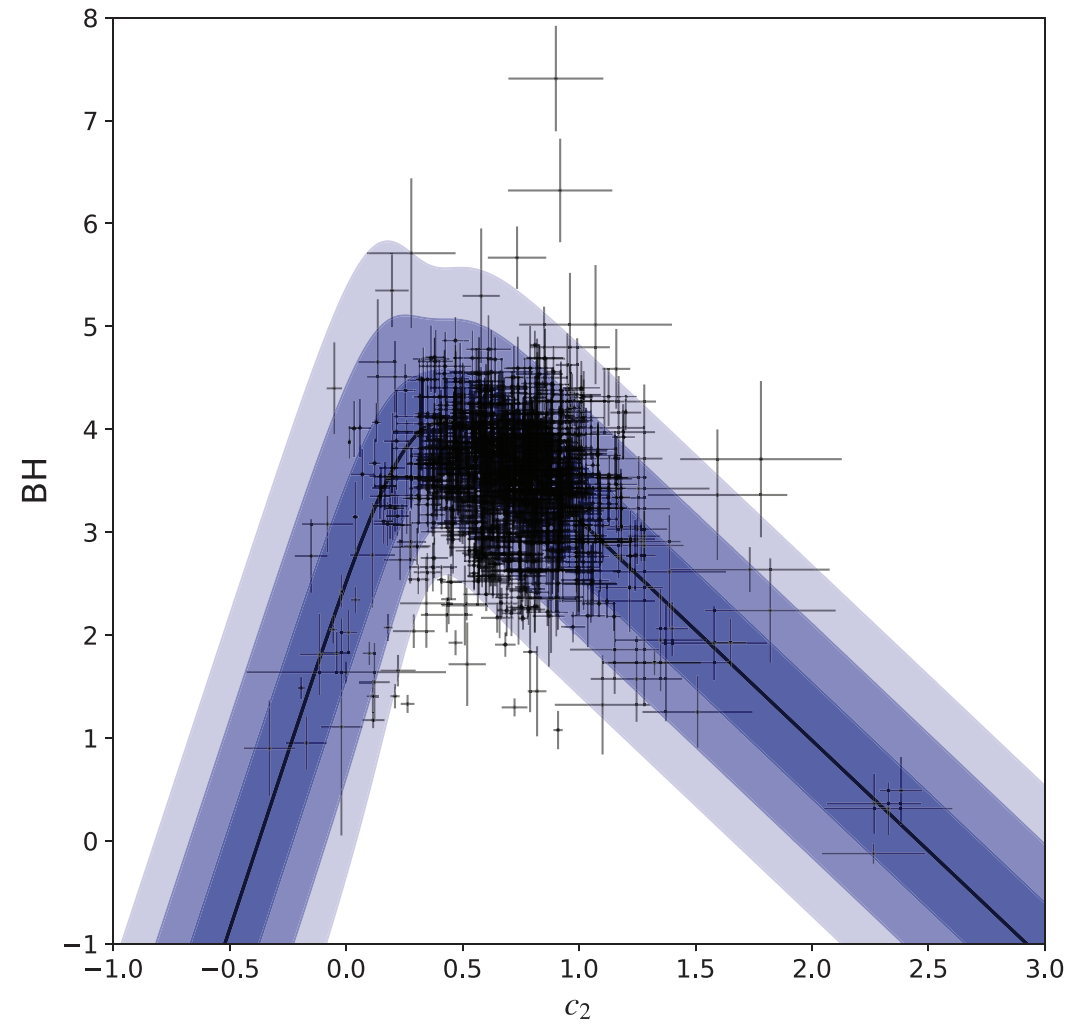
Example "broken-linear" model distribution fit to interstellar extinction model parameter data (see Konz 2020) using the TRK statistic. Shaded regions indicate the 1σ, 2σ and 3σ confidence regions of the model distribution.

TRK is a suite for work-case uncertainty Bayesian Regression in 2D.

Robustly fitting a statistical model to data is a task ubiquitous to practically all data-driven fields, but the more nonlinear, uncertain and/or scattered the dataset is, the more diffcult this task becomes. In the common case of two dimensional models (i.e. one independent variable x and one dependent variable y(x)), datasets with intrinsic uncertainties, or error bars, along both x and y prove diffcult to fit to in general, and if the dataset has some extrinsic uncertainty/scatter (i.e., sample variance) that cannot be accounted for solely by the error bars, the difficulty increases still.

Here, we introduce a novel statistic (the Trotter, Reichart, Konz statistic, or TRK) developed that is advantageous towards model-fitting in this "worst-case data" scenario, especially when compared to other methods.

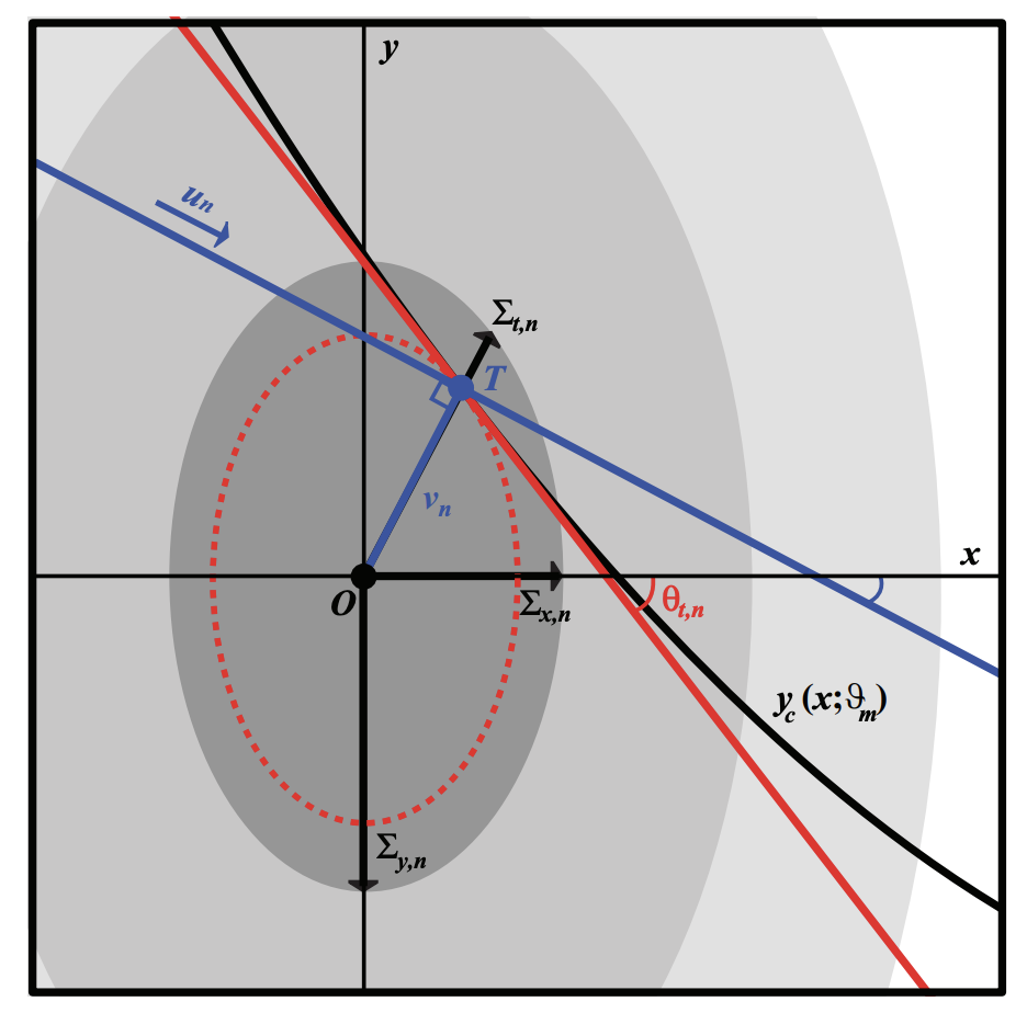
Illustration of the basic geometry of the TRK statistic given a single datapoint and model curve/distribution, from Trotter 2011. The datapoint is centered at (x_n; y_n) (point O), with error ellipse described by the widths (Σ_x,n,Σ_y,n) that combines the intrinsic 2D uncertainty of the datapoint with the extrinsic 2D uncertainty of the model/dataset in general. The model curve y_c(x; θ) is tangent to the error ellipse at tangent point (x_t,n, y_t,n) (point T), and the red line is the linear approximation of the model curve. The blue line indicates the rotated coordinate axis u_n for the TRK statistic (see Konz 2020).)

This statistic, originally introduced in Trotter 2011 is now implemented as a suite of fitting algorithms in C++ that comes equipped with many capabilities, including:

1. Support for any nonlinear model;

2. Probability distribution generation, correlation removal and custom priors for model parameters;

2. Asymmetric 2D uncertainties in the data and/or model, and more.

We also have built a web-based fitting calculator here through which the algorithm can be used easily, but generally, with a high degree of customizability.

The most recent/current documentation and rigorous/thorough introduction of the statistic/the TRK suite is given in Konz 2020. A separate, standalone documentation for the source code itself can be found here.

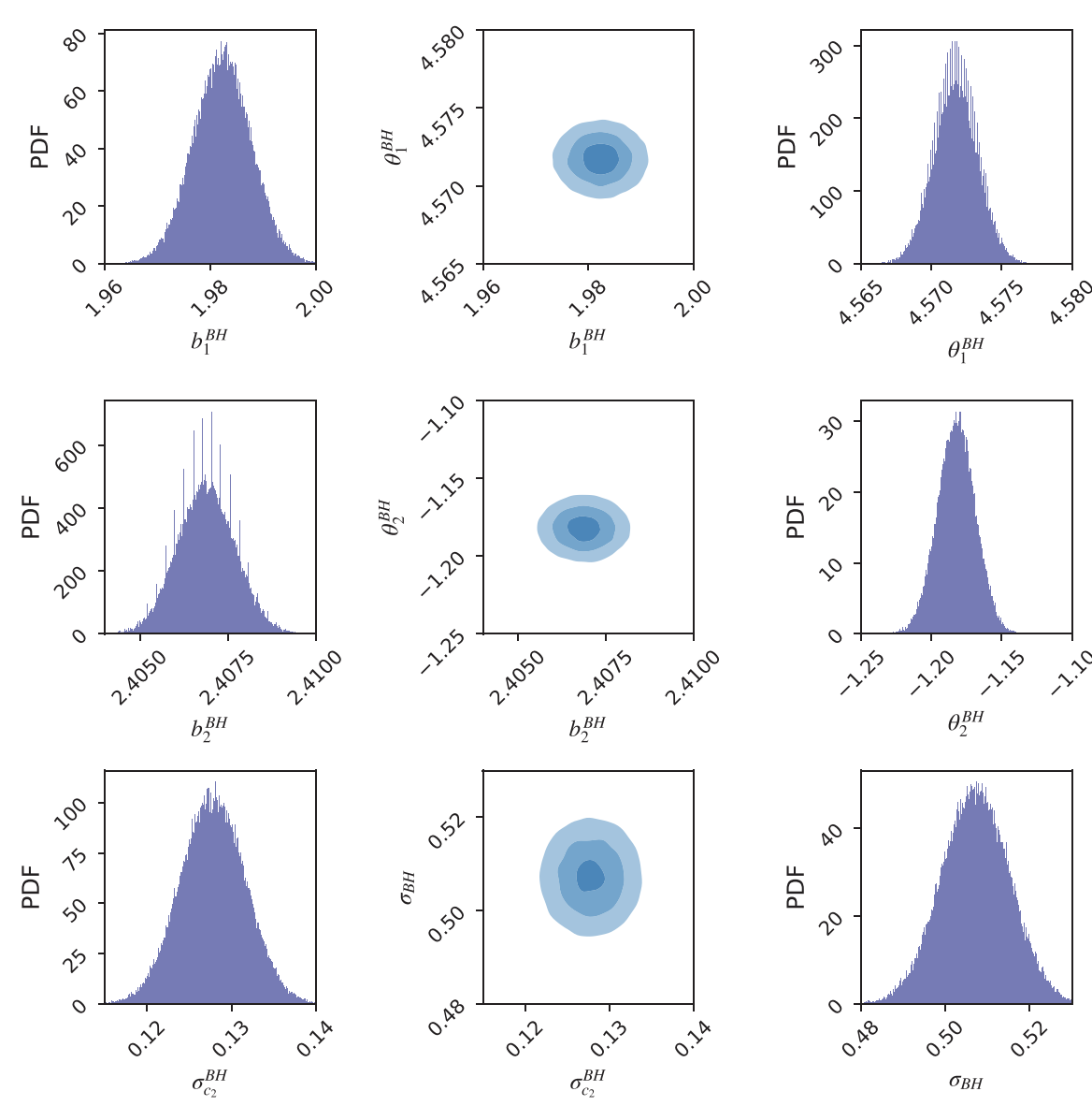
Probability distributions of model and extrinsic variance parameters describing the example "broken-linear" model fit shown in the first figure, generated using Markov Chain-Monte Carlo methods and the TRK statistic. Distributions of individual parameters are along outside columns, while 2D joint distributions are given as confidence ellipses along the center column, with 1σ, 2σ and 3σ confidence regions.

RCR and TRK are free to use for academic and non-commercial applications (licenses here). We only ask that you cite Maples et al. 2018 if using RCR, and Trotter, Reichart and Konz 2020, in preparation if using TRK.

For commercial applications, or consultation, feel free to contact us.